

该数据集中包含三个文件:LC.csv LP.csv LCIS.csv
LC数据集为标的特征表,每只标一条记录。共有21个字段,包括一个主键、7个标本身的信息字段、13个成交时借款人的信息字段。LP数据集为标的还款计划和还款记录表。每只标每期还款一个记录。共有10个字段,包括2个主键,2个还款计划字段和4个还款状态字段。LCIS数据集包含了某一个客户投资的从2015年1月1日起成交的所有标,共36个字段。包含1个主键、7个标自身信息字段和13个成交当时借款人的信息字段以及15个客户投资与收益相关的信息字段。。
二、读取数据集,合并训练集测试集 1.引入库代码如下:
import numpy as np
import pandas as pd
from pandas import Series, Dataframe

import matplotlib.pyplot as plt
%matplotlib inline

# 读取训练数据集
path = r'F:教师培训ppd6PPD-First-Round-Data-UpdatedPPD-First-Round-Data-UpdateTraining Set'

train_loginfo = pd.read_csv(path + 'PPD_LogInfo_3_1_Training_Set.csv', encoding='gbk')
train_master = pd.read_csv(path + 'PPD_Training_Master_GBK_3_1_Training_Set.csv', encoding='gbk')
train_userupdate = pd.read_csv(path + 'PPD_Userupdate_Info_3_1_Training_Set.csv', encoding='gbk')
train_master.shape

# 读取测试数据集
path = 'F:教师培训ppd3PPD-First-Round-Data-UpdateTest Set'
test_loginfo = pd.read_csv(path + 'PPD_LogInfo_2_Test_Set.csv', encoding='gbk')
test_master = pd.read_csv(path + 'PPD_Master_GBK_2_Test_Set.csv', encoding='gb18030')
test_userupdate = pd.read_csv(path + 'PPD_Userupdate_Info_2_Test_Set.csv', encoding='gbk')

# 合并时用于标记哪些样本来自训练集和测试集
train_master['sample_status']='train'
test_master['sample_status']='test'

# 训练集和测试集的合并(axis=0,增加行)
df_Master = pd.concat([train_master,test_master], axis=0).reset_index(drop=True)
df_loginfo = pd.concat([train_loginfo,test_loginfo], axis=0).reset_index(drop=True)
df_userupdate = pd.concat([train_userupdate,test_userupdate], axis=0).reset_index(drop=True)

# 缺失值为-1,替换成nan
df_Master = df_Master.replace({-1:np.nan})
2.缺失值处理
代码如下:
#删除缺失值比例大于0.8的列
plt.figure(figsize=(20,5))
p = (df_Master.isnull().sum().sort_values(ascending=False)/49999).reset_index().rename(columns={'index':'feat_name', 0:'rate'})
df_Master = df_Master.drop(columns=p[p.rate>0.8]['feat_name'])
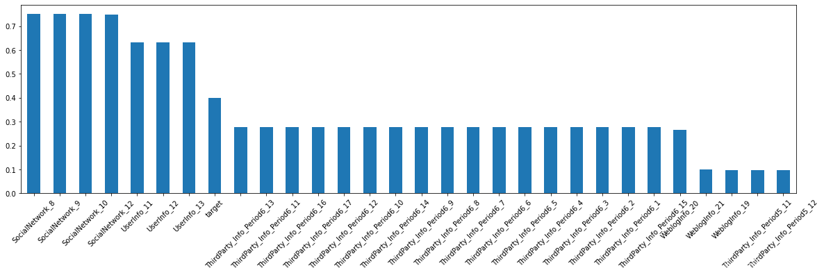
#然后取缺失率排在前30的特征列
plt.figure(figsize=(20,5))
(df_Master.isnull().sum().sort_values(ascending=False)/49999)[:30].plot.bar(rot=45)
#删除缺失数大于100的行
df_Master.isnull().sum(axis=1).sort_values(ascending=True).reset_index(drop=True).plot.line()

a = df_Master.isnull().sum(axis=1).sort_values(ascending=False).reset_index().rename(columns={0:'count_lack_row'})
df_Master = df_Master.drop(index=a[a.count_lack_row>100]['index'])
df_Master.isnull().sum(axis=1).sort_values(ascending=True).reset_index(drop=True).plot.line()

3.将数据集划分为数值类型和类别类型并分别处理
#获取数值类型的特征,并且使用中值填数值类型的特征
b = df_Master.select_dtypes(include=np.float64).drop(columns=['Idx','target'])
for i in b.columns:
b[i].fillna(b[i].median(), inplace=True)
c = b.std().sort_values().reset_index()
c = c.rename(columns={0:'std'})
b = b.drop(columns=c[c['std']<0.1]['index'])
b = pd.concat([b, df_Master[['Idx','target']]],axis=1)
b.head()
#获取类别类型的特征并进行处理
m = df_Master.select_dtypes(include='object')
#统一UserInfo_9数据格式
m.replace({'UserInfo_9':{'中国移动 ':'中国移动', '中国电信 ':'中国电信','中国联通 ':'中国联通'}}, inplace=True)
#统一去掉省,市方便后面操作
m['UserInfo_8'] = m['UserInfo_8'].apply(lambda x: x if x.find('市') == -1 else x[:-1])
m['UserInfo_20'] = m['UserInfo_20'].apply(lambda x: x if x.find('市') == -1 else x[:-1])
m['UserInfo_19'] = m['UserInfo_19'].apply(lambda x: x if x.find('省') == -1 else x[:-1])
m.UserInfo_19.replace({
'广西壮族自治区':'广西',
'宁夏回族自治区':'宁夏',
'新疆维吾尔自治区':'新疆',
'西藏自治区':'西藏',
'内蒙古自治区':'内蒙古'
}, inplace=True)
m['UserInfo_19'] = m['UserInfo_19'].apply(lambda x: x if x.find('市') == -1 else x[:-1])
#对于省份信息UserInfo_7,UserInfo_19筛选出前六名坏人比例比较高的省份,并进行二值化处理,合并到m表
def get_badrate(x):
n = pd.concat([m[x],b['target']],axis=1)
n = n[n['target'].notnull()]
p = (n.groupby(x)['target'].sum()/n.groupby(x)['target'].count()).reset_index()
p = p.rename(columns={x:'province','target':'bad_rate'})
p = p.sort_values('bad_rate',ascending=False)[:6]
return p
#UserInfo_7
p = get_badrate('UserInfo_7')
c = []
for p in p['province']:
c.append('UserInfo_7_is__'+p)
n = pd.get_dummies(m['UserInfo_7'],prefix='UserInfo_7_is_')[c]
m = pd.concat([m,n], axis=1)
# UserInfo_19
p = get_badrate('UserInfo_19')
c = []
for p in p['province']:
c.append('UserInfo_19_is__'+p)
n = pd.get_dummies(m['UserInfo_19'],prefix='UserInfo_19_is_')[c]
m = pd.concat([m,n], axis=1)
#在m表中删除这两个信息
m = m.drop(columns=['UserInfo_7', 'UserInfo_19'])
#接下来对'UserInfo_2','UserInfo_4','UserInfo_8', 'UserInfo_20'这几个城市信息进行处理
# 使用xgboost筛选出重要的城市
from xgboost.sklearn import XGBClassifier
from xgboost import plot_importance
plt.rcParams['font.sans-serif'] = ['Microsoft YaHei']
#将数据哑变量处理后,绘制出重要的城市信息
fig = plt.figure(figsize=(20, 8))
for i, c in enumerate(['UserInfo_2','UserInfo_4','UserInfo_8', 'UserInfo_20']):
k = pd.concat([m[c],b.target],axis=1)
z = pd.get_dummies(k[k.target.notnull()])
ax = fig.add_subplot(2,2,i+1)
clf = XGBClassifier(random_state=0).fit(z.drop(columns='target'), z['target'])
plot_importance(clf,ax=ax,max_num_features=10,height=0.6)

#筛选出重要城市,重新构造特征
k = pd.concat([m['UserInfo_2'],b.target],axis=1)
z = pd.get_dummies(k)
c = []
for p in ['淄博','成都','衡水','梧州','菏泽']:
c.append('UserInfo_2_'+p)
m = pd.concat([m,z[c]], axis=1)
k = pd.concat([m['UserInfo_4'],b.target],axis=1)
z = pd.get_dummies(k)
c = []
for p in ['汕头','梧州','青岛','淄博','成都']:
c.append('UserInfo_4_'+p)
m = pd.concat([m,z[c]], axis=1)
k = pd.concat([m['UserInfo_8'],b.target],axis=1)
z = pd.get_dummies(k)
c = []
for p in ['汕头','梧州','青岛','淄博','成都']:
c.append('UserInfo_8_'+p)
m = pd.concat([m,z[c]], axis=1)
k = pd.concat([m['UserInfo_20'],b.target],axis=1)
z = pd.get_dummies(k)
c = []
for p in ['汕头','梧州','青岛','淄博','成都']:
c.append('UserInfo_20_'+p)
m = pd.concat([m,z[c]], axis=1)
m = pd.concat([m,pd.get_dummies(m['UserInfo_9'])], axis=1)
m.rename(columns={'不详':'未知运营商'}, inplace=True)
#从'UserInfo_2','UserInfo_4','UserInfo_8','UserInfo_20'几个信息中延伸出地址变化次数的特征
m['地址变化次数'] = m[['UserInfo_2','UserInfo_4','UserInfo_8','UserInfo_20']].apply(lambda x:x.nunique(), axis=1)
#删除这些特征
m = m.drop(columns=['UserInfo_2','UserInfo_4','UserInfo_8','UserInfo_9','UserInfo_20'])
#合并特征
df_Master = pd.concat([m,b], axis=1)
#将sample_status这一列,换到最后一列
sample_status = df_Master.pop('sample_status')
df_Master.insert(loc=df_Master.shape[1], column='sample_status', value=sample_status, allow_duplicates=False)
#对于类别类型WeblogInfo_19 WeblogInfo_20 WeblogInfo_21这三列的缺失值用众数填充,然后进行哑变量处理
df_Master.select_dtypes(include='object').isnull().sum()
df_Master.select_dtypes(include='object')[['WeblogInfo_19','WeblogInfo_20','WeblogInfo_21']].mode()
df_Master = df_Master.fillna(value={'WeblogInfo_19':'I','WeblogInfo_20':'I5','WeblogInfo_21':'D'})
df_Master.select_dtypes(include='object').isnull().sum()
#至此第一阶段的特征处理完毕
pd.get_dummies(df_Master[a]).shape
a = ['UserInfo_22', 'UserInfo_23', 'UserInfo_24', 'Education_Info2','Education_Info3', 'Education_Info4', 'Education_Info6',
'Education_Info7', 'Education_Info8', 'WeblogInfo_19', 'WeblogInfo_20','WeblogInfo_21']
b = ['ListingInfo','sample_status']
k = pd.get_dummies(df_Master.drop(columns=b))
df_Master1 = pd.concat([k,df_Master[b]],axis=1)
df_Master1.to_csv(r'F:教师培训ppd6df_Master1.csv', encoding='gb18030')
4.lightGBM进行初步的特征筛选
select = pd.concat([pd.get_dummies(df_Master[a]),df_Master['target']],axis=1)
from sklearn.model_selection import train_test_split
from sklearn.metrics import roc_auc_score,roc_curve,auc
import lightgbm as lgb
from multiprocessing import cpu_count
c = ['target']
x = select[select['target'].notnull()].drop(columns=c)
y = select[select['target'].notnull()]['target']
x_train,x_test, y_train, y_test = train_test_split(x,y,random_state=2,test_size=0.2)
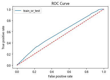
def roc_auc_plot(clf, x, y):
auc = roc_auc_score(y,clf.predict_proba(x)[:,1])
fpr, tpr, _ = roc_curve(y,clf.predict_proba(x)[:,1])
ks = abs(fpr-tpr).max()
print('ks = ', ks)
print('auc = ', auc)
from matplotlib import pyplot as plt
plt.plot(fpr,tpr,label = 'train_or_test')
plt.plot([0,1],[0,1],'k--', c='r')
plt.xlabel('False positive rate')
plt.ylabel('True positive rate')
plt.title('ROC Curve')
plt.legend(loc = 'best')
plt.show()
clf = lgb.LGBMClassifier(
boosting_type='gbdt', num_leaves=31, reg_alpha=0.0, reg_lambda=1,
max_depth=2, n_estimators=800,max_features = 140, objective='binary',
subsample=0.7, colsample_bytree=0.7, subsample_freq=1,
learning_rate=0.05, min_child_weight=50,random_state=None,n_jobs=cpu_count()-1,
num_iterations = 800 #迭代次数
)
clf = clf.fit(x_train, y_train,eval_set=[(x_train, y_train),(x_test,y_test)],eval_metric='auc',early_stopping_rounds=100)
roc_auc_plot(clf, x_test, y_test)
feature = pd.Dataframe(
{'name' : clf.booster_.feature_name(),
'importance' : clf.feature_importances_
}).set_index('name')
mm = feature.sort_values('importance',ascending = False)
kk = mm[mm.importance>0].index.to_list()
a = ['UserInfo_22', 'UserInfo_23', 'UserInfo_24', 'Education_Info2','Education_Info3', 'Education_Info4', 'Education_Info6',
'Education_Info7', 'Education_Info8', 'WeblogInfo_19', 'WeblogInfo_20','WeblogInfo_21']
df_Master2 = pd.concat([df_Master.drop(columns=a),select[kk]], axis=1)
df_Master2.to_csv(r'F:教师培训ppd6df_Master2.csv', encoding='gb18030')
5.lightGBM重新建模
#针对去掉特征的df_Master2进行建模,
from sklearn.model_selection import train_test_split
from sklearn.metrics import roc_auc_score,roc_curve,auc
import lightgbm as lgb
from multiprocessing import cpu_count
import pandas as pd
df_Master2 = pd.read_csv(r'F:教师培训ppd6df_Master2.csv',encoding='gb18030')
df_Master2 = df_Master2.drop(columns='Unnamed: 0')
c = ['target','ListingInfo','sample_status']
x = df_Master2[df_Master2['target'].notnull()].drop(columns=c)
y = df_Master2[df_Master2['target'].notnull()]['target']
x_train,x_test, y_train, y_test = train_test_split(x,y,random_state=2,test_size=0.2)
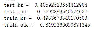
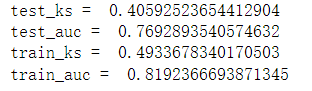
def roc_auc_plot(clf, x_test, y_test, x_train, y_train):
y_pre = clf.predict_proba(x_test)[:,1]
test_auc = roc_auc_score(y_test,y_pre)
test_fpr, test_tpr, _ = roc_curve(y_test,y_pre)
test_ks = abs(test_fpr-test_tpr).max()
print('test_ks = ', test_ks)
print('test_auc = ', test_auc)
y_pre = clf.predict_proba(x_train)[:,1]
train_auc = roc_auc_score(y_train,y_pre)
train_fpr, train_tpr, _ = roc_curve(y_train,y_pre)
train_ks = abs(train_fpr-train_tpr).max()
print('train_ks = ', train_ks)
print('train_auc = ', train_auc)
from matplotlib import pyplot as plt
plt.plot(train_fpr,train_tpr,label = 'train')
plt.plot(test_fpr,test_tpr,label = 'test')
plt.plot([0,1],[0,1],'k--', c='r')
plt.xlabel('False positive rate')
plt.ylabel('True positive rate')
plt.title('ROC Curve')
plt.legend(loc = 'best')
plt.show()
clf = lgb.LGBMClassifier(
boosting_type='gbdt', num_leaves=31, reg_alpha=0.0, reg_lambda=1,
max_depth=2, n_estimators=800,max_features = 140, objective='binary',
subsample=0.7, colsample_bytree=0.7, subsample_freq=1,
learning_rate=0.05, min_child_weight=50,random_state=None,n_jobs=cpu_count()-1,
num_iterations = 800 #迭代次数
)
clf = clf.fit(x_train, y_train,eval_set=[(x_train, y_train),(x_test,y_test)],eval_metric='auc',early_stopping_rounds=100)
roc_auc_plot(clf, x_test, y_test, x_train, y_train)
#针对没有去除特征的df_Master1进行建模
from sklearn.model_selection import train_test_split
from sklearn.metrics import roc_auc_score,roc_curve,auc
import lightgbm as lgb
from multiprocessing import cpu_count
import pandas as pd
df_Master2 = pd.read_csv(r'F:教师培训ppd6df_Master2.csv',encoding='gb18030')
df_Master2 = df_Master2.drop(columns='Unnamed: 0')
c = ['target','ListingInfo','sample_status']
x = df_Master2[df_Master2['target'].notnull()].drop(columns=c)
y = df_Master2[df_Master2['target'].notnull()]['target']
x_train,x_test, y_train, y_test = train_test_split(x,y,random_state=2,test_size=0.2)
clf = lgb.LGBMClassifier(
boosting_type='gbdt', num_leaves=31, reg_alpha=0.0, reg_lambda=1,
max_depth=2, n_estimators=800,max_features = 140, objective='binary',
subsample=0.7, colsample_bytree=0.7, subsample_freq=1,
learning_rate=0.05, min_child_weight=50,random_state=None,n_jobs=cpu_count()-1,
num_iterations = 800 #迭代次数
)
clf = clf.fit(x_train, y_train,eval_set=[(x_train, y_train),(x_test,y_test)],eval_metric='auc',early_stopping_rounds=100)
roc_auc_plot(clf, x_test, y_test, x_train, y_train)
6.对df_userupdate表进行信息特征变换
#统一进行小写处理
df_userupdate['UserupdateInfo1'] = df_userupdate['UserupdateInfo1'].apply(lambda x:x.lower())
#提取info1234信息
# 修改信息表
# 衍生变量:
# 1)最近的修改时间距离成交时间差;
# 2)修改信息总次数
# 3)每种信息修改的次数
# 4)按照日期修改的次数
info1 = df_userupdate.groupby('Idx')['UserupdateInfo1'].count()
df_userupdate['ListingInfo1'] = pd.to_datetime(df_userupdate['ListingInfo1'])
df_userupdate['UserupdateInfo2'] = pd.to_datetime(df_userupdate['UserupdateInfo2'])

info2 = df_userupdate.groupby('Idx')['ListingInfo1'].max()-df_userupdate.groupby('Idx')['UserupdateInfo2'].max()
info2 = info2.apply(lambda x : x.days)

info3 = df_userupdate.pivot_table(index='Idx', columns='UserupdateInfo1', values='UserupdateInfo2', aggfunc={'UserupdateInfo2':'count'}).fillna(0)

# 4)按照日期修改的次数
info4 = df_userupdate.groupby('Idx')['UserupdateInfo2'].nunique()
df_userupdate_info = pd.concat([info1, info2, info3, info4],axis=1)
df_userupdate_info.rename(columns={0:'df_use_update0'}, inplace=True)

#序列化到磁盘
df_userupdate_info.to_csv(r'F:教师培训ppd6df_userupdate_info.csv',encoding='gb18030', index=True)
7.对df_loginfo表进行信息特征变换
# 衍生的变量有
# 1)累计登陆次数
# 2)登陆时间的平均间隔
# 3)最近一次的登陆时间距离成交时间差
df_loginfo['Listinginfo1'] = pd.to_datetime(df_loginfo['Listinginfo1'])
df_loginfo['LogInfo3'] = pd.to_datetime(df_loginfo['LogInfo3'])
info1 = df_loginfo.groupby('Idx')['LogInfo3'].count()
def f(x):
    x = x.sort_values(ascending=True)
    y = x-x.shift()
    p = y.apply(lambda z:z.days)
    res = p.sum()/len(x)
    return round(res, 3)

info2 = df_loginfo.groupby('Idx')['LogInfo3'].apply(f)
info3 = df_loginfo.groupby('Idx')['Listinginfo1'].max() - df_loginfo.groupby('Idx')['LogInfo3'].max()
info3 = info3.apply(lambda x:x.days)
df_loginfo_info = pd.concat([info1, info2, info3], axis=1)
df_loginfo_info.rename(columns={'LogInfo3':'login_info1','LogInfo3':'login_info2',0:'login_info3'}, inplace=True)
df_loginfo_info.to_csv(r'F:教师培训ppd6df_loginfo_info.csv',encoding='gb18030', index=True)
8.合并以上三个表df_loginfo_update_info,df_Master1,df_loginfo_update_info并重新建模
df_Master1 = df_Master1.merge(df_loginfo_update_info, on='Idx')
df_Master2 = pd.read_csv(r'F:教师培训ppd6df_Master2.csv',encoding='gb18030')
df_Master2 = df_Master2.merge(df_loginfo_update_info, on='Idx')
# LGBMClassifier在df_Master2数据集上进行预测达到效果最好,所以依此模型为基础进行预测,修改,调参
from sklearn.model_selection import train_test_split
from sklearn.metrics import roc_auc_score,roc_curve,auc
import lightgbm as lgb
from multiprocessing import cpu_count
import pandas as pd
df_Master2 = pd.read_csv(r'F:教师培训ppd6df_Master2.csv',encoding='gb18030')
df_Master2 = df_Master2.drop(columns='Unnamed: 0')
c = ['target','ListingInfo','sample_status', 'Idx']
x = df_Master2[df_Master2['target'].notnull()].drop(columns=c)
y = df_Master2[df_Master2['target'].notnull()]['target']
x_train,x_test, y_train, y_test = train_test_split(x,y,random_state=2,test_size=0.2)
def roc_auc_plot(clf, x_test, y_test, x_train, y_train):
y_pre = clf.predict_proba(x_test)[:,1]
test_auc = roc_auc_score(y_test,y_pre)
test_fpr, test_tpr, _ = roc_curve(y_test,y_pre)
test_ks = abs(test_fpr-test_tpr).max()
print('test_ks = ', test_ks)
print('test_auc = ', test_auc)
y_pre = clf.predict_proba(x_train)[:,1]
train_auc = roc_auc_score(y_train,y_pre)
train_fpr, train_tpr, _ = roc_curve(y_train,y_pre)
train_ks = abs(train_fpr-train_tpr).max()
print('train_ks = ', train_ks)
print('train_auc = ', train_auc)
from matplotlib import pyplot as plt
plt.plot(train_fpr,train_tpr,label = 'train')
plt.plot(test_fpr,test_tpr,label = 'test')
plt.plot([0,1],[0,1],'k--', c='r')
plt.xlabel('False positive rate')
plt.ylabel('True positive rate')
plt.title('ROC Curve')
plt.legend(loc = 'best')
plt.show()
clf = lgb.LGBMClassifier(
boosting_type='gbdt', num_leaves=31, reg_alpha=0.0, reg_lambda=1,
max_depth=2, n_estimators=800,max_features = 140, objective='binary',
subsample=0.7, colsample_bytree=0.7, subsample_freq=1,
learning_rate=0.05, min_child_weight=50,random_state=None,n_jobs=cpu_count()-1,
num_iterations = 800 #迭代次数
)
clf = clf.fit(x_train, y_train,eval_set=[(x_train, y_train),(x_test,y_test)],eval_metric='auc',early_stopping_rounds=100)
roc_auc_plot(clf, x_test, y_test, x_train, y_train)

9.模型调参
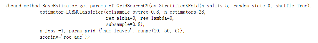
# num_leaves ,步长设为5, 使用网格搜索确定最佳步长
import pandas as pd
from sklearn.model_selection import GridSearchCV, train_test_split
from sklearn.model_selection import cross_val_score
from sklearn.model_selection import StratifiedKFold
import time
import lightgbm as lgb
df_Master2 = pd.read_csv(r'F:教师培训ppd6df_Master2.csv',encoding='gb18030')
df_Master2 = df_Master2.drop(columns='Unnamed: 0')
c = ['target','ListingInfo','sample_status', 'Idx']
x = df_Master2[df_Master2['target'].notnull()].drop(columns=c)
y = df_Master2[df_Master2['target'].notnull()]['target']
x_train,x_test, y_train, y_test = train_test_split(x,y,random_state=2,test_size=0.2)
param_find1 = {'num_leaves':range(10,50,5)}
cv_fold = StratifiedKFold(n_splits=5,random_state=0,shuffle=True)
start = time.time()
grid_search1 = GridSearchCV(estimator=lgb.LGBMClassifier(
learning_rate=0.1,
n_estimators = 28,
max_depth=-1,
min_child_weight=0.001,
min_child_samples=20,
subsample=0.8,
colsample_bytree=0.8,
reg_lambda=0,
reg_alpha=0),
cv = cv_fold,
n_jobs=-1,
param_grid = param_find1,
scoring='roc_auc')
grid_search1.fit(x_train,y_train)
end = time.time()
print('运行时间为:{}'.format(round(end-start,0)))
print(grid_search1.get_params)
print('t')
print(grid_search1.best_params_)
print('t')
print(grid_search1.best_score_)
grid_search1.get_params
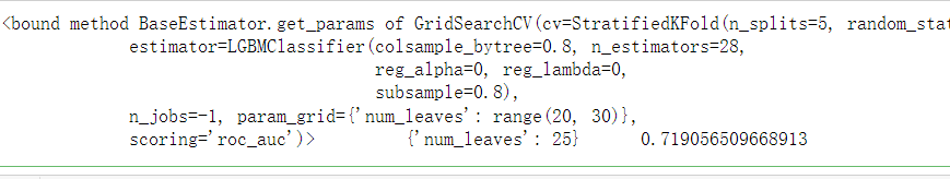
#num_leaves 步长为1
param_find2 = {'num_leaves':range(20,30,1)}
grid_search2 = GridSearchCV(
estimator=lgb.LGBMClassifier(n_estimators=28,
learning_rate=0.1,
min_child_weight=0.001,
min_child_samples=20,
subsample=0.8,
colsample_bytree=0.8,
reg_alpha=0,
reg_lambda=0),
cv=StratifiedKFold(n_splits=5, random_state=0,shuffle=True),
n_jobs=-1,
scoring='roc_auc',
param_grid=param_find2
)
grid_search2.fit(x_train, y_train)
print(grid_search2.get_params,'t',grid_search2.best_params_,'t',grid_search2.best_score_)
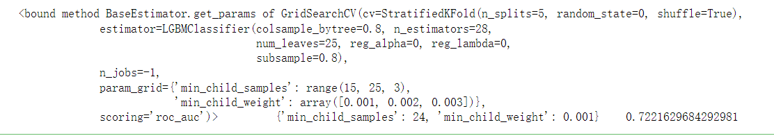
import numpy as np
#确定num_leaves 为25 ,面进行min_child_samples 和 min_child_weight的调参,设定步长为5
param_find3 = {
'min_child_weight':np.linspace(0.001,0.003,3),
'min_child_samples':range(15,25,3)
}
grid_search3 = GridSearchCV(
estimator=lgb.LGBMClassifier(n_estimators=28,
learning_rate=0.1,
num_leaves=25,
subsample=0.8,
colsample_bytree=0.8,
reg_alpha=0,
reg_lambda=0),
cv=StratifiedKFold(n_splits=5, random_state=0,shuffle=True),
n_jobs=-1,
scoring='roc_auc',
param_grid=param_find3
)
grid_search3.fit(x_train, y_train)
print(grid_search3.get_params,'t',grid_search3.best_params_,'t',grid_search3.best_score_)
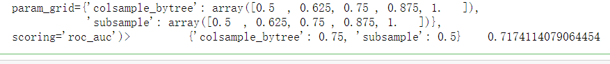
#确定参数{'min_child_samples': 24, 'min_child_weight': 0.001},下面对subsample和colsample_bytree进行调参
param_find4 = {
'subsample':np.linspace(0.5,1,5),
'colsample_bytree':np.linspace(0.5,1,5)
}
grid_search4 = GridSearchCV(
estimator=lgb.LGBMClassifier(n_estimators=28,
learning_rate=0.1,
num_leaves=25,
min_child_weight=0.001,
min_child_samples=24,
# subsample=0.8,
# colsample_bytree=0.8,
reg_alpha=0,
reg_lambda=0),
cv=StratifiedKFold(n_splits=5, random_state=0,shuffle=True),
n_jobs=-1,
scoring='roc_auc',
param_grid=param_find4
)
grid_search4.fit(x_train, y_train)
print(grid_search4.get_params,'t',grid_search4.best_params_,'t',grid_search4.best_score_)
#重新建模
lgb_single_model = lgb.LGBMClassifier(n_estimators=28,
learning_rate=0.11188888888888888,
num_leaves=25,
min_child_weight=0.001,
min_child_samples=24,
subsample=0.5,
colsample_bytree=0.75,
reg_alpha=0.3,
reg_lambda=0.126)
lgb_single_model.fit(x_train,y_train)
pre = lgb_single_model.predict_proba(x_test)[:,1]
acu_curve(y_test,pre)
总结
以上代码参考https://zhuanlan.zhihu.com/p/56864235此文,并加入自己理解和改进,数据集https://www.kesci.com/home/competition/56cd5f02b89b5bd026cb39c9/content/1
